Guido
project 01
How I connected the sensors, motors, and ROS 2 stack behind Guido, with a closer look at getting SLAM to make sense of a moving robot.
Most Innovative Hack @ HackUSF 2026
stack: ROS2, Python, C++, SLAM Toolbox, Nav2, Jetson Orin Nano, Arduino
Building Guido#
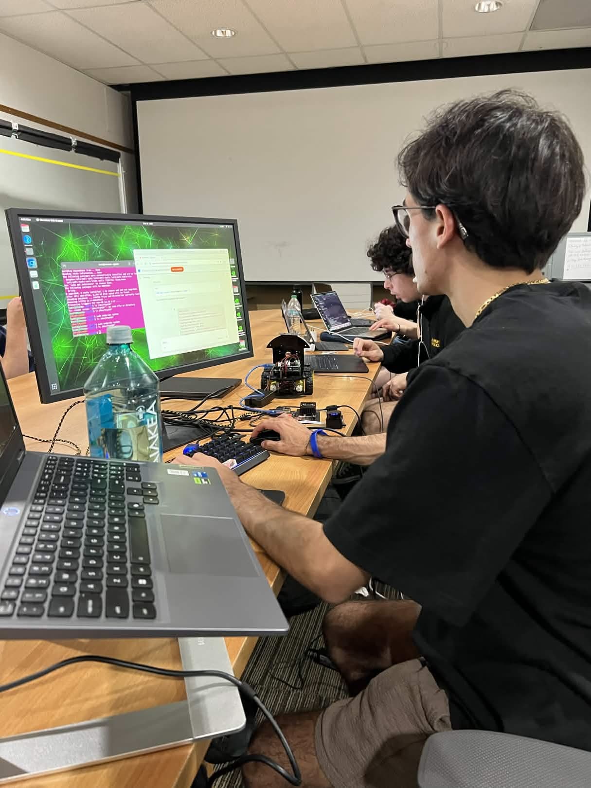
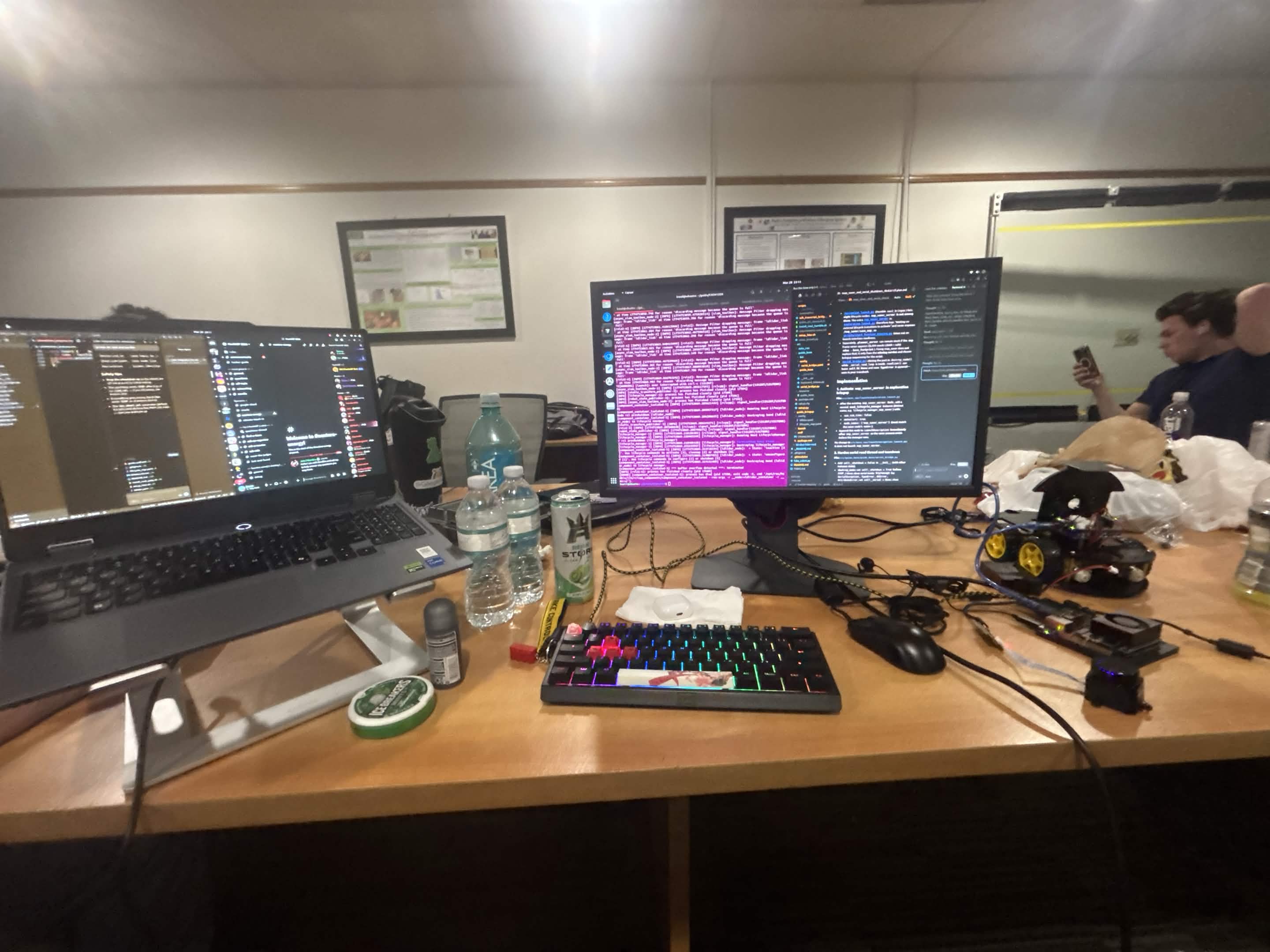
We built Guido at HackUSF 2026: a small robot exploring what a voice-controlled autonomous wheelchair could do. It mapped rooms with LiDAR, navigated to waypoints, and connected spoken commands to physical movement. We ended up winning Most Innovative Hack out of 280+ projects. The Devpost has the team overview, but I want to get into the robotics work here.
My part was getting the hardware talking to ROS 2 and making those messages mean something. If the wheels turn, does the robot's position update correctly? If the LiDAR sees a wall, does that wall stay in the same place when the robot moves? Those questions connect a surprising amount of the stack, from encoder counts on the Arduino all the way up to SLAM and Nav2.
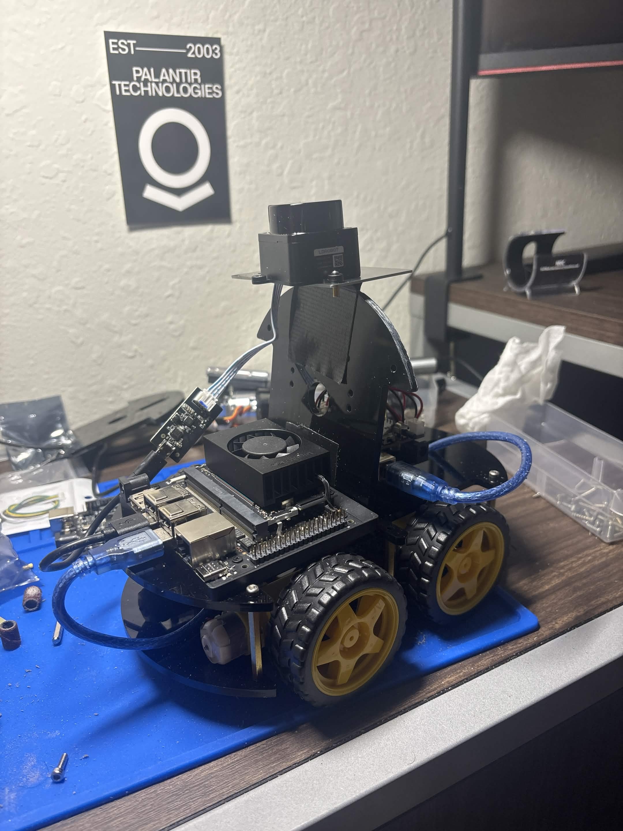
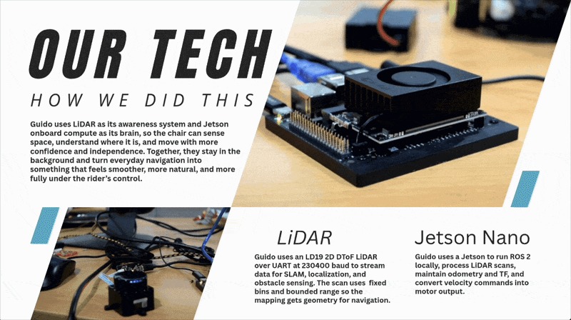
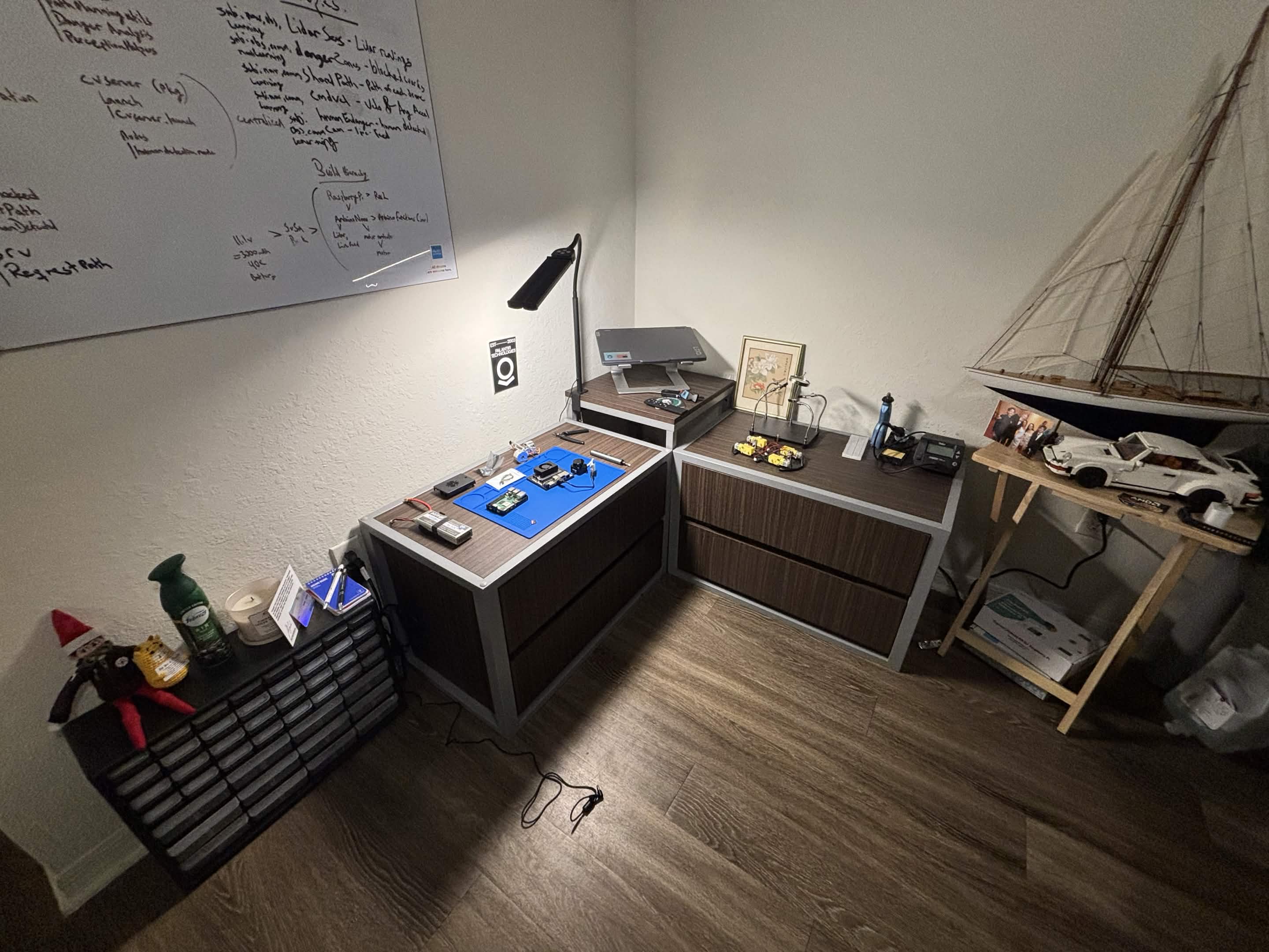
The hardware photo above shows the scale of the prototype. The Jetson Orin Nano 8 GB ran Ubuntu and ROS 2 Humble. The LD19 sat above the chassis, while the Arduino handled the motor interface and sensor readings. This was a research and hackathon platform, not a production or medically validated mobility device.
What I built, and what we built together#
My initial hardware bringup introduced the LiDAR configuration, robot description, launch file, and setup scripts. I then added the motor bridge and Arduino firmware. My later commits on frontier-mapping changed the sensor plumbing, TF ownership, SLAM processing, Nav2 configuration, and the route from navigation commands to the motors.
We split the work across the team. Michael developed the earlier exploration and supervisory architecture. Carlos worked on base bringup, motor direction and PWM calibration, and later the waypoint backend and telemetry frontend. Adrian handled speech and agent integration. Michael's article goes into the exploration side; mine spends more time on the hardware, mapping, and motion underneath it.
If you're following along in GitHub, use the March 29 revision 62f1964. A lot of the overnight work lives on frontier-mapping, beyond where main stops. There are a few different launch paths in there, which I'll keep separate as we go.
From hardware to ROS messages#
The Jetson and Arduino talked over serial. The Jetson handled mapping and navigation; the Arduino handled encoder interrupts, motor direction pins, and PWM. That kept the Arduino's job pretty small: take a wheel command, drive the motor controller, and report motion back. The motor driver handled the electrical side of powering the motors.
| Component | Connection | What it does |
|---|---|---|
| LD19 LiDAR | /dev/ldlidar, 230400 baud | Supplies distance samples to ldlidar::LdLidarComponent |
| LiDAR ROS node | /ldlidar_node/scan, LaserScan | Publishes ranges in ldlidar_link |
| Jetson motor bridge | guido_serial_bridge, 115200 baud | Converts Twist commands into signed wheel PWM; parses returned state |
| Arduino | L<int> R<int> and STOP lines | Sets motor direction and duty cycle; counts encoder pulses; reads gyro Z |
| Odometry return | ODOM x y theta vLin vAng | Becomes /odom and, when enabled, a dynamic TF |
| State estimator | ekf_filter_node | In the frontier launch, publishes /odometry/filtered and the odometry TF |
The LiDAR and motor controller used different serial devices and baud rates. The motor YAML used a /dev/serial/by-id/… path, while the LiDAR setup installed a udev alias. These names help keep a reboot or USB enumeration change from silently swapping which peripheral a node tries to open. Bridge settings and LiDAR setup preserve that boundary.
Velocity is not PWM#
ROS describes chassis motion with geometry_msgs/Twist. For our differential-drive interface, linear.x is forward velocity and angular.z is yaw rate. My bridge splits that request into left and right wheel velocities:
v_left  = v - ωL/2
v_right = v + ωL/2
Here L is the configured wheel separation, 0.17 m. The bridge then divides each wheel velocity by max_wheel_vel = 0.5 m/s, multiplies by 255, converts to an integer, and clamps to the signed PWM range. That 0.5 is a configurable motor-model assumption, not a measured top speed.
The core conversion in the serial bridge is short:
v_left = linear_x - (angular_z * self._wheel_base / 2.0)
v_right = linear_x + (angular_z * self._wheel_base / 2.0)

pwm_left = int(self._clamp(v_left / self._max_wheel_vel * 255.0, -255, 255))
pwm_right = int(self._clamp(v_right / self._max_wheel_vel * 255.0, -255, 255))
Before sending the command, the bridge applies each wheel's direction, gain, and minimum PWM settings. Carlos added those calibration controls. In the late YAML, both wheels have a minimum nonzero PWM of 51. A zero command still stops the motor, but a tiny movement command gets bumped up to that floor.
For a calculated example, requesting v = 0.12 m/s and ω = 0.5 rad/s gives wheel targets of 0.0775 and 0.1625 m/s. The raw integer PWM values are 39 and 82; the configured floor changes them to 51 and 82. This is arithmetic from the code, not a measured drive test. It shows why a locally sensible controller output can change curvature at the motor boundary.
The catch is that the firmware sets PWM and reports motion, without adjusting PWM to hold a target wheel speed. We had encoders, but we didn't have a closed-loop wheel velocity controller in this version. So Nav2 could ask for a particular turn while the motors only approximately followed it. That matters for mapping too, because the motion estimate has to describe the turn the chassis actually made.
How the pieces talk to each other#
The common perception path starts with the LD19 driver. SLAM needs both the scan and a transform relating its sensor frame to the moving base. It publishes the occupancy map and the correction between the map and odometry coordinate systems.
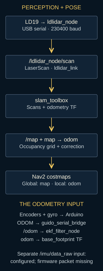
Figure 1. Sensor and pose inputs in frontier_mapping.launch.py. The EKF's additional IMU input is configured, but the checked-in firmware does not emit the separate packet needed to feed it.
The launch file changes how those pieces are connected:
| Launch path | Pose and mapping | Motion execution |
|---|---|---|
auto_nav/slam_teleop.launch.py | Live SLAM; serial bridge owns odometry TF by default | Keyboard commands to /cmd_vel |
auto_nav/navigation.launch.py or slam_nav.launch.py | Live SLAM; base launch defaults to no EKF | Waypoint bridge to Nav2; /cmd_vel_nav through twist_mux |
auto_nav/frontier_mapping.launch.py | Live SLAM; explicitly enables EKF and filtered odometry | Nav2 infrastructure plus a separately started frontier explorer; explorer directly publishes /cmd_vel |
The waypoint command nodes connect /auto_nav/command to /auto_nav/request, then to the /navigate_to_pose action. The speech/agent integration can supply the command text. This is where the team's voice work meets navigation; it does not change the motor protocol.
The late frontier explorer is different. It asks Nav2's /compute_path_to_pose action for a preview, but its drive loop steers toward the frontier itself. It does not follow the returned path through DWB. Its defaults start with human approval; an a key toggles automatic approval. Calling every movement in that branch “Nav2-controlled” would hide an important hackathon compromise. Explorer source.
There is also a separate guido_navigation package with its own perception, planner, trajectory controller, command mux, and safety monitor. Its bringup files are alternatives, not extra stages secretly running inside the Nav2 launch. In particular, /navigation/filtered_scan belongs to that path; the Nav2/SLAM configuration discussed below consumes /ldlidar_node/scan directly.
Frames and odometry: agreeing about motion#
A LiDAR return starts as a distance and angle relative to the sensor. A goal is a pose in the map. A wheel command concerns the chassis. TF connects those descriptions without forcing every subsystem to use one coordinate system.
odom gives the controller a locally continuous motion estimate, even as accumulated error grows. map lets SLAM correct that drift relative to the room. Keeping them separate means a map correction does not have to be treated as an instantaneous physical movement of the wheels.
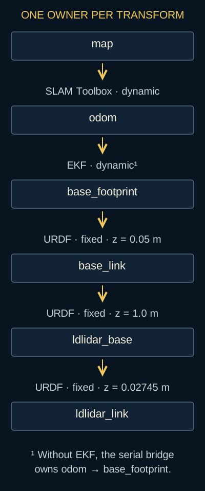
Figure 2. The frontier launch's TF chain. Only one node should own odom → base_footprint. The three fixed links come from guido_state_publisher and the URDF.
The URDF sets base_footprint → base_link to 0.05 m vertically, base_link → ldlidar_base to 1.0 m, and the final sensor offset to 0.02745 m. These are committed model values, not verified physical measurements. The 0.70 × 0.60 m visual body and 1 m mount still resemble a larger wheelchair model, while the late navigation footprint is much smaller. A connected TF tree can still contain wrong geometry.
I consolidated the sensor-frame joint into Guido's URDF and brought up the LiDAR component without the upstream package's separate robot-description publisher. Later, commit cbaf0b2 removed an identity odom → base_footprint fallback from the frontier launch, enabled the EKF, and disabled the serial bridge's TF publication in that mode:
parameters=[
    bridge_config,
    {'publish_tf': not use_ekf},
]
This is an easy thing to get wrong: a transform can exist and still be telling the rest of ROS the wrong thing. The identity fallback says the chassis hasn't moved at all. Leaving it alongside measured motion gives two answers to the same question. There's also a fake_odom.py development helper in the repo, but the final frontier launch doesn't use it.
What the Arduino actually estimates#
The firmware snapshots and resets encoder counts with interrupts disabled. Wheel distance is circumference times pulse count divided by ticks per revolution. It averages the two wheel distances for translation, integrates MPU6050 gyro Z for heading, and updates position along that heading.
The constants are WHEEL_RADIUS = 0.033, WHEEL_BASE = 0.17, and TICKS_PER_REV = 20; the late firmware explicitly labels the geometry and encoder scale as placeholders to measure. Its 50 ms elapsed-time check targets approximately 20 Hz odometry. That is a scheduling intention, not a logged achieved rate.
There is no quadrature direction measurement in this version. Michael's firmware update recovers pulse sign from the most recent commanded wheel direction. That helps represent reverse commands, but cannot reliably identify motion caused by pushing the robot, wheel slip, or a direction reversal while the wheel is still coasting. Gyro bias also accumulates into heading error. These are reasons to use odometry as a short-term estimate, not ground truth.
On the Jetson, the bridge timestamps each parsed packet at receipt. There is no acquisition timestamp in ODOM, so serial delay becomes part of the timing error. The publisher also leaves odometry covariance at message defaults. Neither a valid message type nor an updating RViz pose proves the uncertainty model is calibrated.
The IMU plumbing still had a gap#
I added support for separate IMU ax ay az gx gy gz packets and /imu/data_raw. The bridge marks orientation unavailable and publishes angular velocity and acceleration in base_link; there is no separate IMU frame in this model.
The EKF configuration runs in 2D with a configured 50 Hz output. Its selection masks fuse forward velocity and yaw rate from /odom, plus yaw rate from /imu/data_raw. It does not fuse the Arduino's position fields, an absolute IMU heading, or acceleration.
There's a gap here, though. The firmware in Git only prints ODOM, so the separate IMU input doesn't have a packet producer in this version. Gyro Z already reaches ROS inside the odometry message, but that isn't the same as having both sensor streams hooked up. Finishing the IMU path would also mean checking that the filter isn't treating two copies of the same gyro reading as independent evidence.
Getting SLAM to make sense of the room#
SLAM was where a lot of my hardware work came together. The LiDAR could tell us how far away a surface was, but turning those readings into a room meant knowing where the sensor was when it took them. As soon as the chassis moves, the motor and odometry work becomes part of the mapping problem.
My work here was mostly connecting SLAM Toolbox to our robot and tuning what went into it. SLAM Toolbox supplied the scan matching and mapping machinery. I had to give it scans in the right frame, a usable motion estimate, and settings that made sense for this small chassis on a Jetson.
A scan is still attached to the robot#
The LD19 driver publishes /ldlidar_node/scan as a LaserScan: distances arranged by angle around the sensor. Our LiDAR configuration uses meters, counterclockwise rotation, the ldlidar_link frame, and a fixed 455-bin scan. The driver's source specifically calls out fixed bin counts for SLAM Toolbox compatibility.
Those points are relative to the LiDAR. Say the robot turns next to a wall. The wall hasn't moved, but the distances and angles in the next scan look different because the sensor has rotated. If we just drew every scan at the same origin, we'd be drawing a moving view of the room, not building a map of it.
That's why the frame chain matters. SLAM needs to know where ldlidar_link sits on the chassis and how the chassis moved in odom. A scan can look perfectly reasonable in its own frame while being unusable in the map because one of those relationships is missing or wrong.
The driver accepts ranges from 0.03 to 15 m. Those are configured bounds, not a claim that we measured accurate returns across that whole distance. We also didn't save a measured scan rate, so I won't attach a made-up frequency to the sensor stream.
Why SLAM still needs odometry#
Odometry gives SLAM a starting estimate of how far the robot moved between scans. Scan matching then looks for a pose that makes the new measurements line up with geometry already observed. If both scans saw the same wall, we want those observations to agree about where that wall is.
For Guido, that starting estimate came through the Arduino's encoder and gyro calculations, then the serial bridge and, in frontier mode, the EKF. A wheel-scale error or a drifting heading estimate therefore reaches SLAM before it has even started matching the next scan. Scan matching can correct the estimate, but handing it a worse starting point makes the job harder.
Imagine the chassis moves a short distance while its odometry says it stayed still. The next scan sees the room from somewhere else, but the motion estimate hasn't caught up. That disagreement is the kind of thing I'd check before spending more time adjusting the scan matcher. This is an explanation of the failure mode, not a claim that we recorded that exact event.
The correction lives in map → odom. The local odometry frame can keep following motion continuously while SLAM adjusts how that frame sits in the room. This is also why removing the static odometry fallback mattered: the rest of the system needed an estimate that could actually move with the robot.
What gets drawn into the map#
SLAM Toolbox publishes /map as an occupancy grid. Each cell describes whether that part of the room is free, occupied, or still unknown. Our resolution: 0.05 means a cell is 5 cm across. It doesn't mean we localized the robot to within 5 cm.
A valid range return gives evidence of a surface at its endpoint and free space along the observed ray before it. Space behind that surface hasn't been observed through it. That sounds obvious, but it's important when looking at a partly built map: a blank or unknown area isn't automatically a place the robot can drive.
The global planner was configured to allow unknown cells, and the explorer used the boundary between free and unknown space to propose new destinations. Both depend on what the map actually says. If the base pose is wrong, the resulting map can misplace obstacles before navigation gets a chance to reason about them.
There are also several different update rates here. A new scan, a new TF message, and a refreshed occupancy grid are different events. The late configuration publishes the map on a 3-second interval and the map-to-odometry transform on a 0.05-second period. That doesn't mean SLAM solves a new map twenty times a second. It means consumers can receive the current transform more often than the full grid is refreshed.
Nav2 also reads live scans into its obstacle layers, so it doesn't have to wait for the next full SLAM map to receive a nearby obstacle observation. Getting that distinction right helps explain why a map display and a local costmap might update differently.
The settings I actually changed#
The late auto_nav/config/slam_toolbox.yaml runs async_slam_toolbox_node in mapping mode. These were the settings that mattered most to the integration:
| Parameter | Value | What I was controlling |
|---|---|---|
resolution | 0.05 m | How finely the occupancy grid divides the room |
max_laser_range | 6.0 m | How far out to use returns for mapping |
throttle_scans | 3 | How aggressively to subsample scans before the other checks |
minimum_time_interval | 0.5 s | A minimum time gap between accepted scans |
minimum_travel_distance | 0.15 m | The translation threshold used in scan processing |
minimum_travel_heading | 0.1 rad | The angular motion threshold in the mapping configuration |
transform_publish_period | 0.05 s | How often to publish the current map-to-odometry transform |
map_update_interval | 3.0 s | How often to refresh the occupancy grid |
loop_match_minimum_chain_size | 10 | How much matching scan-chain support to require for loop closure |
These values weren't all settled at the beginning. The history shows a fairly clear back-and-forth on how much data to process:
| Setting | Before 02:23 | At 02:23 | At 07:02 |
|---|---|---|---|
throttle_scans | 1 | 5 | 3 |
minimum_time_interval | 0.25 s | 0.5 s | 0.5 s |
map_update_interval | 2 s | 5 s | 3 s |
minimum_travel_distance | 0.05 m | 0.05 m | 0.15 m |
minimum_travel_heading | 0.05 rad | 0.05 rad | 0.1 rad |
At 02:23, I cut back the scan processing and map refresh rate. That commit also reduced the odometry and IMU publisher queue depths to 2, and the motor-command subscriber depth to 1.
The tradeoff is pretty practical. Keeping every message sounds good until the robot is moving and you're working through old information. Processing fewer scans gives up some observations, but also asks less of the system. Smaller queues limit how much old data those ROS endpoints can hold. Neither setting fixes every possible delay, especially with a serial connection further down the chain.
At 07:02, I brought the scan throttle back to 3 and the map interval to 3 seconds. I also increased the movement thresholds. The comments in that change call out stationary jitter: if the robot hasn't meaningfully changed position, tiny differences between scans can add noise without giving much new information about the room.
Those gates interact. Passing the scan-throttle check doesn't mean a scan passes the time and motion checks too. For a sense of scale, traveling 0.15 m at Nav2's configured 0.12 m/s takes 1.25 seconds. That's arithmetic from the settings, not an observed update rate, but it shows why a 0.5-second time gate doesn't mean the map gains a new observation every half second.
I don't have a before/after latency trace or mapping-error measurement for these changes. The commits show what I adjusted and the comments explain the concerns. They don't let me put a percentage improvement next to the result.
Range limits and loop closure#
In that same 07:02 change, I reduced max_laser_range from 12 to 6 m. The comment describes keeping the mapping range useful for indoor rooms. A longer sensor range isn't automatically more useful for every map; it also brings more distant observations into the problem. The appropriate cutoff depends on the space and the quality of those returns.
I also tried to exclude returns closer than 15 cm because the configuration comments call out the robot body and wheel reflections. Looking back at the file, there's a catch: it says minimum_laser_range: 0.15, while the upstream Humble code reads min_laser_range. I can't count that entry as a working filter without checking the exact installed version and its runtime parameters. It's a good example of a setting looking right in the file while potentially doing nothing.
Loop closure addresses a different problem. As the robot travels, small pose errors can accumulate. When it sees a place again, matching that revisit to an earlier observation gives SLAM another constraint on how the map fits together. Done correctly, that helps keep a room consistent across a longer path.
Accepting the wrong match is a problem too. I increased loop_match_minimum_chain_size from 6 to 10; the comment says this was intended to reduce false closures in sparse early maps. Requiring more supporting scans makes the acceptance more demanding, but can also make a useful closure harder to obtain. The configured search distance stayed at 3 m. Again, that's the tuning tradeoff visible in the source, not a measured loop-closure success rate.
Saving the map, then finding yourself in it again#
The explorer calls nav2_map_server's map_saver_cli to write frontier_map.pgm and a YAML file with the map metadata. The image records the occupancy grid. The metadata tells a later consumer how to place that image in coordinates.
That isn't all the information SLAM used to build it. Saving an occupancy image is different from serializing SLAM Toolbox's pose graph, which preserves the connected scan-and-pose history needed for its continued-mapping or localization workflow. Having a saved floor plan also doesn't tell a restarted robot where it currently sits inside that floor plan.
The early branch had separate SLAM mapping and localization YAML files. The late Nav2 path discussed here keeps mapping live. Another launch, guido_autonomy.launch.py, can enable a map server and AMCL with use_amcl and map_yaml. AMCL estimates the robot's pose against the existing map; that configuration uses a likelihood-field laser model and 250 to 1500 particles. It belongs to the custom navigation path and consumes its filtered scan, so I wouldn't mix it into the frontier-mode diagram.
We didn't preserve a generated Guido map or serialized pose graph in the audited repository. The LiDAR dependency includes example maps, but those aren't ours. I'd rather explain the actual map pipeline than put someone else's room in the article and imply we mapped it.
Getting Nav2 commands onto the drivetrain#
In the waypoint path, auto_nav_navigation_node turns a stored pose into a NavigateToPose goal. The behavior-tree navigator coordinates planning and control. The configured global planner is NavFn with A* enabled. It searches the global costmap for a route; the DWB local planner evaluates short candidate motions against the local costmap and path-related critics.
Global planning answers how to get across the mapped room. Local control answers which motion is feasible now, including when a new object appears in front of the chassis. DWB's configured critics include ObstacleFootprint, PathAlign, PathDist, GoalAlign, GoalDist, and RotateToGoal. Their weights trade path tracking and goal progress against other trajectory costs. Nav2 parameters.
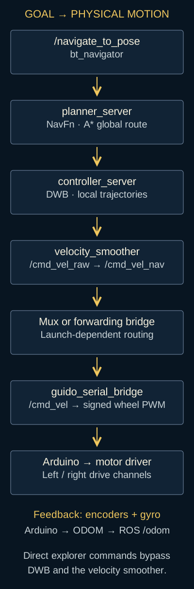
Figure 3. Configured Nav2 execution path. The waypoint launch uses twist_mux; the frontier infrastructure uses nav_cmd_vel_bridge. The explorer's direct commands bypass DWB and the velocity smoother.
My Nav2 launch remaps controller output to /cmd_vel_raw, then routes velocity_smoother output to /cmd_vel_nav. Recovery behaviors publish to /cmd_vel_nav directly. In the waypoint launch, twist_mux gives /cmd_vel_teleop priority 20 and navigation priority 10. In frontier bringup, the forwarding bridge passes /cmd_vel_nav to the motor bridge's /cmd_vel input.
The launch includes a lifecycle manager for the controller, path smoother, planner, behaviors, navigator, waypoint follower, and velocity smoother. A node appearing in the graph is not enough: a lifecycle node must be configured and activated before it provides its intended service. The YAML points at Humble's navigate_w_replanning_time.xml behavior tree. The path smoother server and the velocity smoother are different things: one operates on path geometry, the other on velocity commands.
Numbers that eventually reach the wheels#
| Nav2 setting | Late value | Meaning for the robot |
|---|---|---|
| Controller frequency | 10 Hz | Target cadence for choosing local motion |
DWB max_vel_x / max_vel_theta | 0.12 m/s / 0.5 rad/s | Bounds on the controller's forward and turning requests |
DWB acc_lim_x / acc_lim_theta | 0.2 m/s² / 0.6 rad/s² | Acceleration assumptions used for candidate motion |
DWB decel_lim_x / decel_lim_theta | -0.25 m/s² / -0.6 rad/s² | Deceleration limits in the model |
DWB sim_time | 1.2 s | Prediction horizon for candidate trajectories |
| DWB velocity samples | 12 linear, 20 angular | Sampling density for candidate commands |
| Goal checker | 0.15 m, 0.5 rad | Position and orientation acceptance tolerances |
| Progress checker | 0.05 m within 25 s | Minimum movement before declaring insufficient progress |
| Velocity smoother | 10 Hz, OPEN_LOOP | Smooths commands from command history, not measured velocity feedback |
Even with those limits, the command still has to get through the PWM conversion. The smoother can produce a gradual change in velocity while the minimum PWM setting turns part of it into a jump. That's why looking at /cmd_vel alone only tells part of the story.
The goal checker's angular tolerance changed from 0.35 to 0.5 rad, roughly 20 to 29 degrees, while position tolerance changed from 0.12 to 0.15 m. That accepts a less exact final pose. The planner's separate tolerance changed from 0.5 to 1.0 m, permitting a wider search for a reachable endpoint near the requested goal. These are distinct tolerances, and neither should be described as demonstrated positioning accuracy.
Costmaps and the size of the robot#
The global costmap uses the map frame and combines a static map layer with live obstacles and inflation. The local costmap uses odom, rolls with the robot, and covers 4 × 4 m. Both have 0.05 m cells. The local scan source marks obstacles out to 2.5 m and raytraces clearing observations out to 3 m; globally those bounds are 5 and 6 m.
Marking inserts occupied observations. Clearing uses observed rays to remove obstacles where the sensor now sees through a previously occupied area. Inflation assigns cost around obstacles so planning can prefer clearance instead of merely avoiding the exact hit cell.
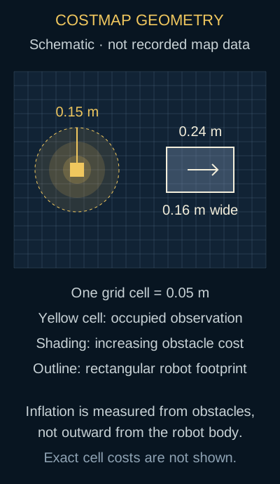
Figure 4. Geometry derived from the late Nav2 YAML. The illustration is not a recorded map or an exact reproduction of Nav2's discrete cost values.
At 07:02 I changed both footprints from a 0.70 × 0.60 m rectangle to 0.24 × 0.16 m, and reduced inflation radius from 0.35 to 0.15 m. The inflation cost-scaling factor changed from 5 to 3. A smaller footprint changes which passages count as traversable; it is not just an RViz cosmetic adjustment.
The new footprint extends 12 cm forward/backward and 8 cm to either side of the base origin. Its circumscribed radius is about 14.4 cm, calculated from the corner coordinates, so the 15 cm inflation radius is fairly tight. Inflation radius is measured from obstacle cells; it is not an extra 15 cm of guaranteed clearance outside the chassis. The footprint collision checks still matter.
I changed the navigation geometry toward the small chassis, but didn't bring every representation into agreement. The URDF still has the larger visual body. There's no saved measurement sheet or corridor test behind these numbers, so I'd remeasure both before trusting the clearance model.
Where the late demo path bypasses those limits#
The explorer's final direct-drive loop requests 0.10 m/s forward speed and uses heading error with optional IMU yaw-rate damping. It checks a forward LiDAR sector of ±25 degrees and stops below 0.30 m. It stops if it cannot obtain the robot's map-frame pose.
Its angular command cap is 19.0 rad/s, far above Nav2's 0.5 rad/s. That is a software request bound, not a measured turn rate. Because it publishes directly to /cmd_vel, Nav2's smoother cannot enforce its limits on that path; the serial bridge instead saturates wheel PWM. The loop also treats a missing scan as infinite obstacle distance and does not check scan age. This is narrower protection than the separate custom safety-monitor node offers, and that node is not launched here.
Those details explain why I would not present the final explorer as a polished obstacle-avoiding Nav2 controller. Planning a valid preview, steering toward a goal, and safely tracking the planned route are different capabilities.
When the individual pieces work but the robot doesn't#
The saved runtime log gives a less tidy picture than the diagrams. There's a LiDAR launch trying to find a standalone executable that isn't there, FastRTPS shared-memory open_and_lock_file errors, failed lifecycle startup, and the global costmap waiting for a map frame that doesn't exist yet. These were problems before the robot even got to the interesting part of navigation.
The later source loads ldlidar::LdLidarComponent into component_container_isolated, matching the driver's actual packaging. The frontier launch selects a UDP-only FastRTPS transport profile, with a comment connecting it to discovery failures on the Jetson. Those are concrete responses preserved in code. The log does not isolate one root cause for every failed launch, nor provide a controlled rerun proving each change independently fixed the problem.
A missing map transform is especially easy to misdiagnose as a planner problem. The costmap cannot place the robot in the global map until SLAM has a usable scan and odometry chain. Increasing a planner tolerance does not create that missing transform.
The repository's verify_nav_motion script checks /cmd_vel, samples /odom, looks for /odometry/filtered, and asks TF for map → base_footprint. That gives a useful order for diagnosis:
- Confirm the sensor and serial nodes are active and publishing fresh data.
- Check the actual frame names and motion transform, not only a visible point cloud.
- Verify that the map and costmaps represent the chassis at a sensible scale.
- Follow a command through its remapped topics to the serial bridge.
- Compare the requested movement with what the wheels and odometry report.
- Change the responsible layer and repeat the physical test.
The configured RViz views expose scans, maps, TF, robot geometry, and frontier/path previews. They help compare what ROS believes with the robot on the floor. They do not measure wheel slip or prove a footprint is correct.
A lot of this came down to checking one connection at a time. Seeing a motor spin doesn't tell you whether its encoder scale is right. Seeing odometry arrive doesn't tell you whether its timestamp is useful. I needed those checks to agree with the robot on the floor before treating the map or planner as the thing to fix.
What we got working#
We got a physical prototype mapping with LiDAR, navigating to waypoints, avoiding obstacles, and responding to voice-driven movement and navigation commands. That was the team's demo, and it won Most Innovative Hack at HackUSF 2026. Michael's writeup covers those results from his side too.
For me, the interesting part was the connection between wheel motion and the map. The Arduino could report movement, ROS could place the sensor relative to the chassis, and SLAM could use that information to map the room. The different navigation paths then used that map and pose to request more movement. There were still rough edges in that loop, as the source makes pretty clear.
What I would change with more time#
The first priority would be making measured motion match commanded motion. I would calibrate wheel radius, encoder scale, wheel separation, sensor placement, and the footprint against the physical chassis. Then I would use direction-aware encoders and closed-loop wheel velocity control, characterize motor deadband, and collect commanded-versus-measured traces. That would make navigation tuning depend on observed drivetrain behavior instead of a PWM approximation.
I would finish the IMU packet path, use acquisition timestamps, calibrate the gyro, and assign defensible covariance values. The EKF inputs should contribute independent information where possible. I would also reconcile the remaining URDF geometry and verify each parameter against the exact installed ROS package version.
For navigation, I would consolidate the launch variants and enforce one motion-arbitration and stop path. The direct explorer should either execute its planned route through the navigation controller or have its own tested trajectory and collision logic. Missing or stale obstacle data should stop motion. A valid preview should never stand in for validating the command actually sent to the motors.
The bridge already sends STOP after 0.5 s without a command, and the later firmware includes a 500 ms command timeout. Those mechanisms help with interrupted command delivery, but the firmware checks its timeout inside a loop that also performs blocking serial reads. They are not a hard real-time stopping guarantee or independent emergency-stop system.
A full-sized device carrying a person would require a different level of engineering: independent emergency stopping and braking, redundant fault handling, validated sensing coverage, measured stopping behavior under load, and extensive supervised testing across surfaces and failure conditions. The hackathon prototype did not establish any of that.
Guido made me pay much more attention to what sits underneath a map. A wall on the screen depends on an actual sensor reading, a frame, a timestamp, and an estimate of how the robot moved. I spent a lot of my part of the project getting those pieces connected. Next time, I'd record their data from the start so I could put the physical robot and the ROS estimate side by side instead of relying so heavily on what I could see in RViz.